ELECTRIC SHOCK

Sabado, Enero 3, 2015

Impedance and Admittance

Susceptance and Admittance

Admittance (symbolized Y ) is an expression of the ease with which alternating current ( AC ) flows through a complex circuit or system. Admittance is a vector quantity comprised of two independent scalar phenomena: conductance and susceptance .

Impedance, denoted Z, is an expression of the opposition that an electronic component, circuit, or system offers to alternating and/or direct electric current.Impedance is a vector (two-dimensional)quantity consisting of two independent scalar (one-dimensional) phenomena: resistance and reactance.

In the study of DC circuits, the student of electricity comes across a term meaning the opposite of resistance: conductance. It is a useful term when exploring the mathematical formula for parallel resistances: Rparallel = 1 / (1/R1 + 1/R2 + . . . 1/Rn). Unlike resistance, which diminishes as more parallel components are included in the circuit, conductance simply adds. Mathematically, conductance is the reciprocal of resistance, and each 1/R term in the “parallel resistance formula” is actually a conductance.

Whereas the term “resistance” denotes the amount of opposition to flowing electrons in a circuit, “conductance” represents the ease of which electrons may flow. Resistance is the measure of how much a circuit resists current, while conductance is the measure of how much a circuit conducts current. Conductance used to be measured in the unit of mhos, or “ohms” spelled backward. Now, the proper unit of measurement is Siemens. When symbolized in a mathematical formula, the proper letter to use for conductance is “G”.

Reactive components such as inductors and capacitors oppose the flow of electrons with respect to time, rather than with a constant, unchanging friction as resistors do. We call this time-based opposition, reactance, and like resistance we also measure it in the unit of ohms.

As conductance is the complement of resistance, there is also a complementary expression of reactance, called susceptance. Mathematically, it is equal to 1/X, the reciprocal of reactance. Like conductance, it used to be measured in the unit of mhos, but now is measured in Siemens. Its mathematical symbol is “B”, unfortunately the same symbol used to represent magnetic flux density.

The terms “reactance” and “susceptance” have a certain linguistic logic to them, just like resistance and conductance. While reactance is the measure of how much a circuit reacts against change in current over time, susceptance is the measure of how much a circuit is susceptible to conducting a changing current

Series-parallel R, L, and C

Now that we've seen how series and parallel AC circuit analysis is not fundamentally different than DC circuit analysis, it should come as no surprise that series-parallel analysis would be the same as well, just using complex numbers instead of scalar to represent voltage, current, and impedance.

Take this series-parallel circuit for example: (Figure below)

Sinusoids and Phasors

A Sinusoid is a signal that has the form of the sine or cosine function.

A sinusoidal current is usually referred to as alternating current (ac).
Such a current reverses at regular time intervals and has alternately pos-
itive and negative values. Circuits driven by sinusoidal current or volt-
age sources are called ac circuits.

A sinusoidal forcing function produces both a transient response
and a steady-state response, much like the step function, which we stud-
ied in Chapters 7 and 8. The transient response dies out with time so
that only the steady-state response remains. When the transient response
has become negligibly small compared with the steady-state response,
we say that the circuit is operating at sinusoidal steady state. It is this
sinusoidal steady-state response.

A sinusoid having period T and angular frequency

can be represented as

A periodic function is one that satisﬁes f (t) f (tnT), for all t and
for all integers n.

Basically a rotating vector, simply called a “Phasor” is a scaled line whose length represents an AC quantity that has both magnitude (“peak amplitude”) and direction (“phase”) which is “frozen” at some point in time.

A phasor is a vector that has an arrow head at one end which signifies partly the maximum value of the vector quantity ( V or I ) and partly the end of the vector that rotates.

Polar representation: $z = \vert z\vert\;e^{j\angle z}$ , or simply $z=\vert z\vert\;\angle z$ , where $\vert z\vert$ and $\angle z$ are the magnitude and phase angle, respectively.

The two representations can be converted from one to the other:

From to $(\vert z\vert,\angle z)$ :

$\begin{displaymath}\left\{ \begin{array}{ll} \vert z\vert=\sqrt{x^2+y^2} & \mbox... ...gle z=tan^{-1} (y/x) & \mbox{phase angle} \end{array} \right. \end{displaymath}$
From $(\vert z\vert,\angle z)$ to :

$\begin{displaymath}z=\vert z\vert\;e^{j\angle z}=\vert z\vert(\cos\angle z+j\;\sin\angle z)=x+jy \end{displaymath}$

due to Euler identity, i.e.,

$\begin{displaymath}\left\{ \begin{array}{ll} x=\vert z\vert\;\cos\angle z & \mbo... ...ert\;\sin\angle z & \mbox{imaginary part} \end{array} \right. \end{displaymath}$

The arithmetic operations of two complex numbers $z=x+jy=\vert z\vert\;e^{j\angle z}$ and $w=u+jv=\vert w\vert\;e^{j\psi}$ are listed below:

Add/Subtract:

$\begin{displaymath}z+w=(x+u)+j(y+v),\;\;\;\;z-w=(x-u)+j(y-v) \end{displaymath}$
Multiply:

$\begin{displaymath}z\;w=(x+jy)(u+jv)=(xu-yv)+j(xv+yu)=\vert z\vert\;\vert w\vert\;e^{j(\angle z+\angle w)} \end{displaymath}$
Divide:

$\begin{displaymath}\frac{z}{w}=\frac{x+jy}{u+jv}=\frac{(x+jy)(u-jv)}{(u+jv)(u-jv... ... =\frac{\vert z\vert}{\vert w\vert}\;e^{j(\angle z-\angle w)} \end{displaymath}$

Sabado, Oktubre 4, 2014

Maximum Power Transfer

The Maximum Power Transfer Theorem is not so much a means of analysis as it is an aid to system design. Simply stated, the maximum amount of power will be dissipated by a load resistance when that load resistance is equal to the Thevenin/Norton resistance of the network supplying the power. If the load resistance is lower or higher than the Thevenin/Norton resistance of the source network, its dissipated power will be less than maximum.

This is essentially what is aimed for in radio transmitter design , where the antenna or transmission line “impedance” is matched to final power amplifier “impedance” for maximum radio frequency power output. Impedance, the overall opposition to AC and DC current, is very similar to resistance, and must be equal between source and load for the greatest amount of power to be transferred to the load. A load impedance that is too high will result in low power output. A load impedance that is too low will not only result in low power output, but possibly overheating of the amplifier due to the power dissipated in its internal (Thevenin or Norton) impedance.

The Maximum Power Transfer Theorem states that the maximum amount of power will be dissipated by a load resistance if it is equal to the Thevenin or Norton resistance of the network supplying power.

The Maximum Power Transfer Theorem does not satisfy the goal of maximum efficiency.

Maximum Power Transfer Example No1.

Where:
  RS = 25Ω
  RL is variable between 0 – 100Ω
  VS = 100v

Then by using the following Ohm’s Law equations:

We can now complete the following table to determine the current and power in the circuit for different values of load resistance.

Table of Current against Power

RL (Ω)	I (amps)	P (watts)
0	4.0	0
5	3.3	55
10	2.8	78
15	2.5	93
20	2.2	97

RL (Ω)	I (amps)	P (watts)
25	2.0	100
30	1.8	97
40	1.5	94
60	1.2	83
100	0.8	64

Using the data from the table above, we can plot a graph of load resistance, RL against power, P for different values of load resistance. Also notice that power is zero for an open-circuit (zero current condition) and also for a short-circuit (zero voltage condition).

Graph of Power against Load Resistance

Norton's Theorem

Norton's Theorem states that it is possible to simplify any linear circuit, no matter how complex, to an equivalent circuit with just a single current source and parallel resistance connected to a load. Just as with Thevenin's Theorem, the qualification of “linear” is identical to that found in the Superposition Theorem: all underlying equations must be linear (no exponents or roots).

Contrasting our original example circuit against the Norton equivalent: it looks something like this:

Remember that a current source is a component whose job is to provide a constant amount of current, outputting as much or as little voltage necessary to maintain that constant current.

As with Thevenin's Theorem, everything in the original circuit except the load resistance has been reduced to an equivalent circuit that is simpler to analyze. Also similar to Thevenin's Theorem are the steps used in Norton's Theorem to calculate the Norton source current (INorton) and Norton resistance (RNorton).

Norton's Theorem is a way to reduce a network to an equivalent circuit composed of a single current source, parallel resistance, and parallel load.

Steps to follow for Norton's Theorem:

(1) Find the Norton source current by removing the load resistor from the original circuit and calculating current through a short (wire) jumping across the open connection points where the load resistor used to be.
(2) Find the Norton resistance by removing all power sources in the original circuit (voltage sources shorted and current sources open) and calculating total resistance between the open connection points.
(3) Draw the Norton equivalent circuit, with the Norton current source in parallel with the Norton resistance. The load resistor re-attaches between the two open points of the equivalent circuit.
(4) Analyze voltage and current for the load resistor following the rules for parallel circuits.

Example:

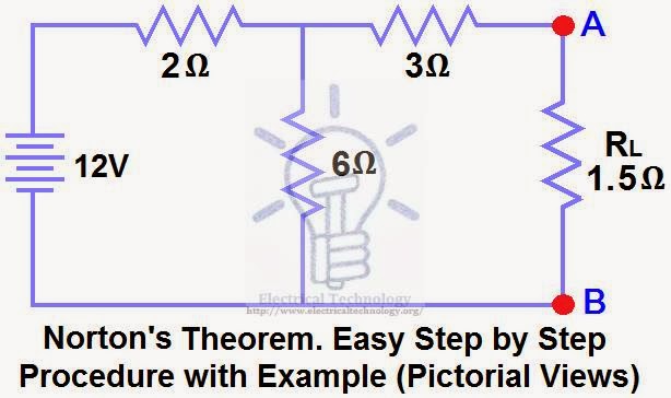
Find R_N, I_N, the current flowing through and Load Voltage across the load resistor in fig (1) by using Norton’s Theorem.

Click image to enlarge

Solution:-

Step 1

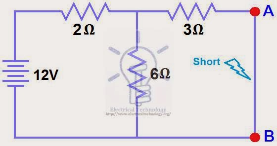
Short the 1.5Ω load resistor as shown in (Fig 2)

Click image to enlarge

Step 2

Calculate / measure the Short Circuit Current. This is the Norton Current (I_N).

We have shorted the AB terminals to determine the Norton current, I_N. The 6Ω and 3Ω are then in parallel and this parallel combination of 6Ω and 3Ω are then in series with 2Ω.

So the Total Resistance of the circuit to the Source is:-

2Ω + (6Ω || 3Ω) ….. (|| = in parallel with)

R_T= 2Ω + [(3Ω x 6Ω) / (3Ω + 6Ω)] → I_T= 2Ω + 2Ω = 4Ω

R_T= 4Ω

I_T = V / R_T

I_T = 12V / 4Ω

I_T = 3A..

Now we have to find I_SC = I_N… Apply CDR… (Current Divider Rule)…

I_SC = I_N = 3A x [(6Ω / (3Ω + 6Ω)] = 2A.

I_SC= I_N= 2A

Click image to enlarge

Step 3

Open Current Sources, Short Voltage Sources and Open Load Resistor. Fig (4)

Click image to enlarge

Step 4

Calculate /measure the Open Circuit Resistance. This is the Norton Resistance (R_N)

We have Reduced the 12V DC source to zero is equivalent to replace it with a short in step (3), as shown in figure (4) We can see that 3Ω resistor is in series with a parallel combination of 6Ω resistor and 2Ω resistor. i.e.:

3Ω + (6Ω || 2Ω) ….. (|| = in parallel with)

R_N = 3Ω + [(6Ω x 2Ω) / (6Ω + 2Ω)]

R_N = 3Ω + 1.5Ω

R_N = 4.5Ω

Click image to enlarge

Step 5

Connect the R_N in Parallel with Current Source I_Nand re-connect the load resistor. This is shown in fig (6) i.e. Norton Equivalent circuit with load resistor.

Click image to enlarge

Norton’s Theorem. Easy Step by Step Procedure with Example (Pictorial Views)

Step 6

Now apply the last step i.e. calculate the load current through and Load voltage across load resistor by Ohm’s Law as shown in fig 7.

Load Current through Load Resistor…

I_L = I_N x [R_N / (R_N+ R_L)]

= 2A x (4.5Ω /4.5Ω +1.5kΩ) → = 1.5A

I_L = 1. 5A

And

Load Voltage across Load Resistor…

V_L = I_L x R_L

V_L = 1.5A x 1.5Ω

V_L= 2.25V

Click image to enlarge

Thevenin's Theorem

Thevenin's Theorem states that it is possible to simplify any linear circuit, no matter how complex, to an equivalent circuit with just a single voltage source and series resistance connected to a load. The qualification of “linear” is identical to that found in the Superposition Theorem, where all the underlying equations must be linear (no exponents or roots). If we're dealing with passive components (such as resistors, and later, inductors and capacitors), this is true. However, there are some components (especially certain gas-discharge and semiconductor components) which are nonlinear: that is, their opposition to current changes with voltage and/or current. As such, we would call circuits containing these types of components, nonlinear circuits.

Thevenin's Theorem is a way to reduce a network to an equivalent circuit composed of a single voltage source, series resistance, and series load.

Steps to follow for Thevenin's Theorem:

(1) Find the Thevenin source voltage by removing the load resistor from the original circuit and calculating voltage across the open connection points where the load resistor used to be.
(2) Find the Thevenin resistance by removing all power sources in the original circuit (voltage sources shorted and current sources open) and calculating total resistance between the open connection points.
(3) Draw the Thevenin equivalent circuit, with the Thevenin voltage source in series with the Thevenin resistance. The load resistor re-attaches between the two open points of the equivalent circuit.
(4) Analyze voltage and current for the load resistor following the rules for series circuits.

Example:

Find V_TH, R_THand the load current flowing through and load voltage across the load resistor in fig (1) by using Thevenin’s Theorem.

Click image to enlarge

Thevenin's Theorem. Easy Step by Step Procedure with Example (Pictorial Views)

1.Open the 5kΩ load resistor

2.Calculate / measure the Open Circuit Voltage. This is the Thevenin Voltage (V_TH). Fig (3)

We have already removed the load resistor from figure 1, so the circuit became an open circuit as shown in fig 2. Now we have to calculate the Thevenin’s Voltage. Since 3mA Current flows in both 12kΩ and 4kΩ resistors as this is a series circuit because current will not flow in the 8kΩ resistor as it is open.

So 12V (3mA x 4kΩ) will appear across the 4kΩ resistor. We also know that current is not flowing through the 8kΩ resistor as it is open circuit, but the 8kΩ resistor is in parallel with 4k resistor. So the same voltage (i.e. 12V) will appear across the 8kΩ resistor as 4kΩ resistor. Therefore 12V will appear across the AB terminals. So,

V_TH = 12V

3. Open Current Sources and Short Voltage Sources. Fig (4)

Click image to enlarge

4.Calculate /measure the Open Circuit Resistance. This is the Thevenin Resistance (R_TH)

We have Reduced the 48V DC source to zero is equivalent to replace it with a short in step (3), as shown in figure () We can see that 8kΩ resistor is in series with a parallel connection of 4kΩ resistor and 12k Ω resistor. i.e.:

8kΩ + (4k Ω || 12kΩ) ….. (|| = in parallel with)

R_TH = 8kΩ + [(4kΩ x 12kΩ) / (4kΩ + 12kΩ)]

R_TH = 8kΩ + 3kΩ

R_TH = 11kΩ

Click image to enlarge

5. Connect the R_THin series with Voltage Source V_TH and re-connect the load resistor. This is shown in fig (6) i.e. Thevenin circuit with load resistor.

Click image to enlarge

6. Now apply the last step i.e. calculate the total load current & load voltage as shown in fig 6.

I_L = V_TH/ (R_TH + R_L)

= 12V / (11kΩ + 5kΩ) → = 12/16kΩ

I_L= 0.75mA

And

V_L = I_Lx R_L

V_L = 0.75mA x 5kΩ

V_L= 3.75V

Click image to enlarge